Programming/Deep Learning

Deep Learning

Introduction

Deep learning (also known as deep structured learning or hierarchical learning) is part of a broader family of machine learning methods based on learning data representations, as opposed to task-specific algorithms. Learning can be supervised, semi-supervised or unsupervised.

There is a massive amount of possible applications where Deep Learning can be deployed, these include:

• Automatic speech recognition
• Image recognition
• Visual art processing
• Natural language processing
• Drug discovery and toxicology
• Customer relationship management
• Recommendation systems
• Bioinformatics
• Health diagnostics
• Image restoration
• Financial fraud detection

There are 6 Types of Artificial Neural Networks Currently Being:

• Recurrent Neural Network(RNN) – Long Short-Term Memory
• Convolutional Neural Network
• Feedforward Neural Network – Artificial Neuron
• Radial basis function Neural Network
• Kohonen Self-Organizing Neural Network
• Modular Neural Network

The top two are the most used.

Introduction to Machine Learning vs Deep Learning

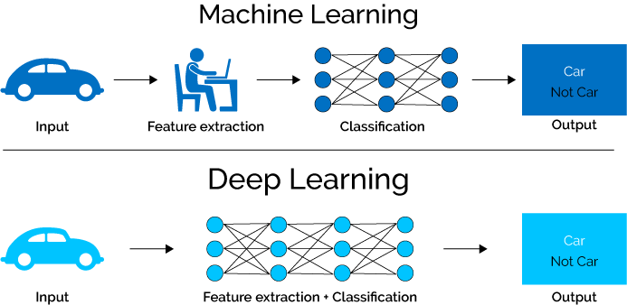
Before starting let us have a look at the two different terms which are Machine Learning and Deep Learning which are closely related. The following diagram shows pictorially the key difference:

With Machine Learning the approach works as the top half of the picture above. You would have to design a feature extraction algorithm that generally involved a lot of heavy mathematics (complex design), wasn’t very efficient, and didn’t perform too well at all (accuracy level just wasn’t suitable for real-world applications). After doing all of that you would also have to design a whole classification model to classify your input given the extracted features.

With Deep Learning networks we can perform feature extraction and classification in one shot, which means we only have to design one model. This also means that with have a lot more layers (usually) and parameters to refine our model to an optimal point.

Machine Learning

• + Good results
• + Quick to train
• - Need to try different features and classifiers to achieve best results
• - Accuracy plateaus

Deep Learning

• + Learns features and classifiers automatically
• + Accuracy is unlimited
• - Requires very large data sets
• - Computationally intensive / expensive

Introduction to Python and its libraries

Python is a general-purpose high-level programming language that is widely used in data science and for producing deep learning algorithms. This brief tutorial introduces Python and its libraries like Numpy, TensorFlow.

Deep structured learning or hierarchical learning or deep learning in short is part of the family of machine learning methods which are themselves a subset of the broader field of Artificial Intelligence.

Machine learning deals with a wide range of concepts. The concepts are listed below −

• supervised
• unsupervised
• reinforcement learning
• linear regression
• cost functions
• overfitting
• under-fitting
• hyper-parameter, etc.

In supervised learning, we learn to predict values from labelled data. One ML technique that helps here is classification, where target values are discrete values; for example, cats and dogs. Another technique in machine learning that could come of help is regression. Regression works on the target values. The target values are continuous values; for example, the stock market data can be analysed using Regression.

Introduction to Neural Network

A typical neural network has anything from a few dozen to hundreds, thousands or even millions of artificial neurons called units arranged in a series of layers, each of which connects to the layers on either side. Some of them, known as input units, are designed to receive various forms of information from the outside world that the network will attempt to learn about, recognise, or otherwise process. Other units sit on the opposite side of the network and signal how it responds to the information it's learned; those are known as output units. In between the input units and output, units are one or more layers of hidden units, which, together, form most of the artificial brain. Most neural networks are fully connected, which means each hidden unit and each output unit are connected to every unit in the layers on either side. The connections between one unit and another are represented by a number called a weight, which can be either positive (if one unit excites another) or negative (if one unit suppresses or inhibits another). The higher the weight, the more influence one unit has on another. (This corresponds to the way actual brain cells trigger one another across tiny gaps called synapses.)

Information flows through a neural network in two ways. When it's learning (being trained) or operating normally (after being trained), patterns of information are fed into the network via the input units, which trigger the layers of hidden units, and these, in turn, arrive at the output units. This common design is called a feedforward network. Not all units "fire" all the time. Each unit receives inputs from the units to its left, and the inputs are multiplied by the weights of the connections they travel along. Every unit adds up all the inputs it receives in this way and (in the simplest type of network) if the sum is more than a certain threshold value, the unit "fires" and triggers the units it's connected to (those on its right).

For a neural network to learn, there has to be an element of feedback involved—just as children learn by being told what they're doing right or wrong. In fact, we all user feedback, all the time. Think back to when you first learned to play a game like ten-pin bowling. As you picked up the heavy ball and rolled it down the alley, your brain watched how quickly the ball moved and the line it followed and noted how close you came to knocking down the skittles. Next time it was your turn, you remembered what you'd done wrong before, modified your movements accordingly, and hopefully threw the ball a bit better. So you used feedback to compare the outcome you wanted with what actually happened, figured out the difference between the two, and used that to change what you did next time ("I need to throw it harder," "I need to roll slightly more to the left," "I need to let go later," and so on). The bigger the difference between the intended and actual outcome, the more radically you would have altered your moves.

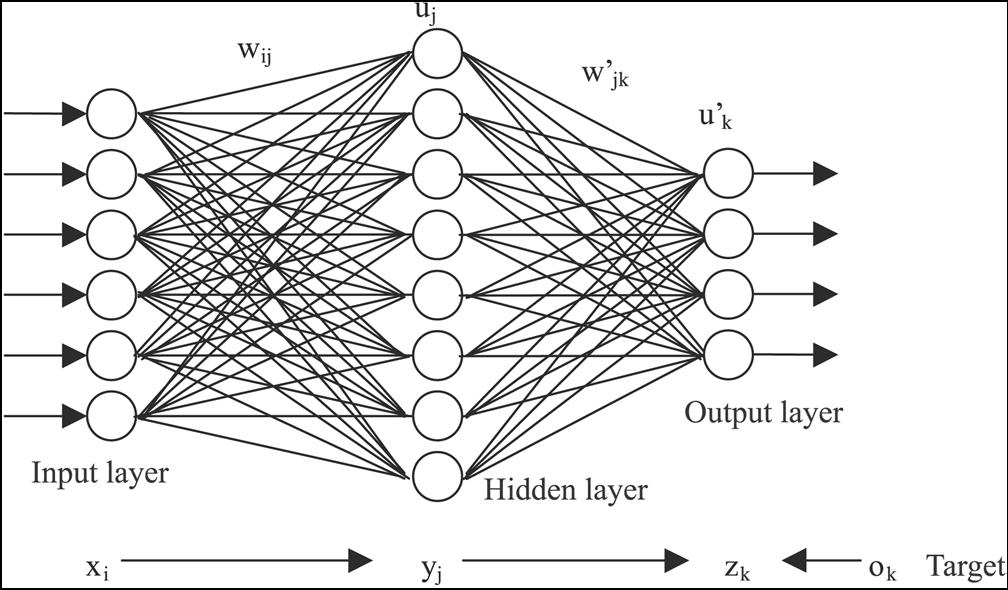
Below shows a neural network example with inputs on the left, a hidden layer, and an output layer. In code, we will try to mimic this theory.

• input layer: brings the initial data into the system for further processing by subsequent layers of artificial neurons.
• hidden layer: a layer in between input layers and output layers, where artificial neurons take in a set of weighted inputs and produce an output through an activation function.
• output layer: the last layer of neurons that produces given outputs for the program.

An artificial neural network consists of artificial neurons or processing elements and is organised in three interconnected layers: input, hidden which may include more than one layer and output.

The input layer contains input neurons that send information to the hidden layer. The hidden layer sends data to the output layer. Every neuron has weighted inputs (synapses), an activation function (defines the output given an input), and one output. Synapses are the adjustable parameters that convert a neural network to a parameter system.

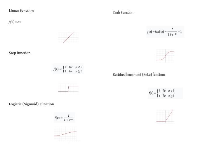
The weighted sum of the inputs produces the activation signal that is passed to the activation function to obtain one output from the neuron. The commonly used activation functions are linear, step, sigmoid, tanh, and rectified linear unit (ReLu) functions.

Neural networks learn things in exactly the same way, typically by a feedback process called back-propagation (sometimes abbreviated as "backprop"). This involves comparing the output a network produces with the output it was meant to produce and using the difference between them to modify the weights of the connections between the units in the network, working from the output units through the hidden units to the input units—going backwards, in other words. In time, back-propagation causes the network to learn, reducing the difference between actual and intended output to the point where the two exactly coincide, so the network figures things out exactly as it should.

Gradient Descent

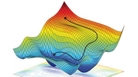
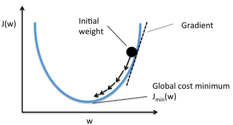
Gradient descent has an analogy of looking for the easiest way down a mountainside, you're going to look for the most gentle way down. In reality, it is a highly mathematical function but for most programmers this is hidden.

From the programming point of view, gradient descent is an iterative method. We start with some sets of values for our model parameters (weights and biases) and improve them slowly.

To improve a given set of weights, we try to get a sense of the value of the cost function (described below) for weights similar to the current weights (by calculating the gradient). Then we move in the direction which reduces the cost function.

By repeating this step thousands of times, we’ll continually minimise our cost function.

On gradients and gradient learning algorithms, the main optimisation technique is used to fit neural network weights to training data sets.

This includes the important distinction between batch and stochastic gradient descent, and approximations via mini-batch gradient descent, today all are simply referred to as stochastic gradient descent.

• Batch Gradient Descent. The gradient is estimated using all examples in the training data set.
• Stochastic (Online) Gradient Descent. The gradient is estimated using subsets of samples in the training data set.
• Mini-Batch Gradient Descent. The gradient is estimated using every single pattern in the training data set.

The mini-batch variant is offered as a way to achieve the speed of convergence offered by stochastic gradient descent with the improved estimate of the error gradient offered by batch gradient descent.

• Larger batch sizes slow down convergence.
• Smaller batch sizes offer a regularising effect due to the introduction of statistical noise in the gradient estimate.

Loss and accuracy

Deep learning neural networks are trained using the stochastic gradient descent optimisation algorithm.

As part of the optimisation algorithm, the error for the current state of the model must be estimated repeatedly. This requires the choice of an error function, conventionally called a loss function, that can be used to estimate the loss of the model so that the weights can be updated to reduce the loss on the next evaluation.

The maths function Mean Square Error (MSE) is the most commonly used regression loss function. MSE is the sum of squared distances between our target variable and predicted values.

Neural network models learn a mapping from inputs to outputs from examples and the choice of loss function must match the framing of the specific predictive modelling problem, such as classification or regression. Further, the configuration of the output layer must also be appropriate for the chosen loss function.

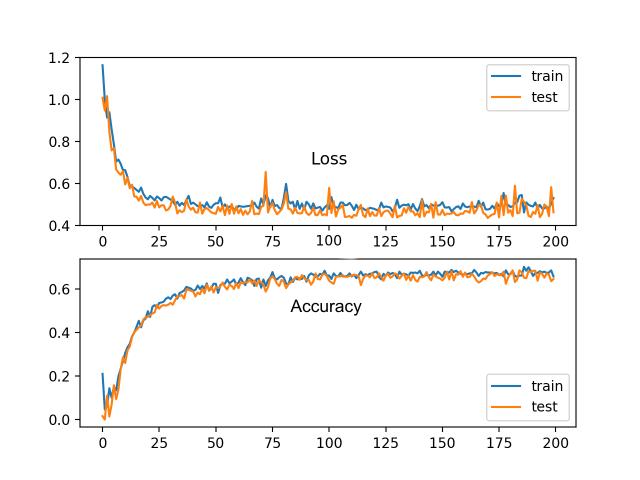
As we keep applying training data to our neural network model we need to measure how close we are to achieving our goal, with a suitable model we should describe something like the following:

Tensorflow

• https://www.tensorflow.org/

Google's TensorFlow Version 2 is a python library, as of version 2 the library Keras is built into the library together with eager execution.

This library is a great choice for building commercial-grade deep-learning applications.

TensorFlow grew out of another library DistBelief V2 which was a part of the Google Brain Project. This library aims to extend the portability of machine learning so that research models could be applied to commercial-grade applications.

Much like the Theano library, TensorFlow is based on computational graphs where a node represents persistent data or math operation and edges represent the flow of data between nodes, which is a multidimensional array or tensor; hence the name TensorFlow

The output from an operation or a set of operations is fed as input into the next.

Even though TensorFlow was designed for neural networks, it works well for other nets where computation can be modelled as a data flow graph.

TensorFlow also uses several features from Theano such as common and sub-expression elimination, auto differentiation, and shared and symbolic variables.

Different types of deep nets can be built using TensorFlow like convolutional nets, Autoencoders, RNTN, RNN, RBM, DBM/MLP and so on.

MNIST Dataset Overview

This example is using MNIST handwritten digits. The dataset contains 60,000 examples for training and 10,000 examples for testing. The digits have been size-normalized and centred in a fixed-size image (28x28 pixels) with values from 0 to 255.

In this example, each image will be converted to float32, normalized to [0, 1] and flattened to a 1-D array of 784 features (28*28).

from __future__ import absolute_import, division, print_function

import tensorflow as tf
from tensorflow.keras import Model, layers
import numpy as np

 MNIST dataset parameters.
num_classes = 10 # total classes (0-9 digits).
num_features = 784 # data features (img shape: 28*28).

# Training parameters.
learning_rate = 0.1
training_steps = 2000
batch_size = 256
display_step = 100

# Network parameters.
n_hidden_1 = 128 # 1st layer number of neurons.
n_hidden_2 = 256 # 2nd layer number of neurons.

# Prepare MNIST data.
from tensorflow.keras.datasets import mnist
(x_train, y_train), (x_test, y_test) = mnist.load_data()
# Convert to float32.
x_train, x_test = np.array(x_train, np.float32), np.array(x_test, np.float32)
# Flatten images to 1-D vector of 784 features (28*28).
x_train, x_test = x_train.reshape([-1, num_features]), x_test.reshape([-1, num_features])
# Normalize images value from [0, 255] to [0, 1].
x_train, x_test = x_train / 255., x_test / 255.

 Use tf.data API to shuffle and batch data.
train_data = tf.data.Dataset.from_tensor_slices((x_train, y_train))
train_data = train_data.repeat().shuffle(5000).batch(batch_size).prefetch(1)
 Create TF Model.
class NeuralNet(Model):
    # Set layers.
    def __init__(self):
        super(NeuralNet, self).__init__()
        # First fully-connected hidden layer.
        self.fc1 = layers.Dense(n_hidden_1, activation=tf.nn.relu)
        # First fully-connected hidden layer.
        self.fc2 = layers.Dense(n_hidden_2, activation=tf.nn.relu)
        # Second fully-connecter hidden layer.
        self.out = layers.Dense(num_classes)

    # Set forward pass.
    def call(self, x, is_training=False):
        x = self.fc1(x)
        x = self.fc2(x)
        x = self.out(x)
        if not is_training:
            # tf cross entropy expect logits without softmax, so only
            # apply softmax when not training.
            x = tf.nn.softmax(x)
        return x

# Build neural network model.
neural_net = NeuralNet()

# Cross-Entropy Loss.
# Note that this will apply 'softmax' to the logits.
def cross_entropy_loss(x, y):
    # Convert labels to int 64 for tf cross-entropy function.
    y = tf.cast(y, tf.int64)
    # Apply softmax to logits and compute cross-entropy.
    loss = tf.nn.sparse_softmax_cross_entropy_with_logits(labels=y, logits=x)
    # Average loss across the batch.
    return tf.reduce_mean(loss)

# Accuracy metric.
def accuracy(y_pred, y_true):
    # Predicted class is the index of highest score in prediction vector (i.e. argmax).
    correct_prediction = tf.equal(tf.argmax(y_pred, 1), tf.cast(y_true, tf.int64))
    return tf.reduce_mean(tf.cast(correct_prediction, tf.float32), axis=-1)

# Stochastic gradient descent optimizer.
optimizer = tf.optimizers.SGD(learning_rate)
# Optimization process. 
def run_optimization(x, y):
    # Wrap computation inside a GradientTape for automatic differentiation.
    with tf.GradientTape() as g:
        # Forward pass.
        pred = neural_net(x, is_training=True)
        # Compute loss.
        loss = cross_entropy_loss(pred, y)
        
    # Variables to update, i.e. trainable variables.
    trainable_variables = neural_net.trainable_variables

    # Compute gradients.
    gradients = g.gradient(loss, trainable_variables)
    
    # Update W and b following gradients.
    optimizer.apply_gradients(zip(gradients, trainable_variables))

# Run training for the given number of steps.
for step, (batch_x, batch_y) in enumerate(train_data.take(training_steps), 1):
    # Run the optimization to update W and b values.
    run_optimization(batch_x, batch_y)
    
    if step % display_step == 0:
        pred = neural_net(batch_x, is_training=True)
        loss = cross_entropy_loss(pred, batch_y)
        acc = accuracy(pred, batch_y)
        print("step: %i, loss: %f, accuracy: %f" % (step, loss, acc))

step: 100, loss: 2.031049, accuracy: 0.535156
step: 200, loss: 1.821917, accuracy: 0.722656
step: 300, loss: 1.764789, accuracy: 0.753906
step: 400, loss: 1.677593, accuracy: 0.859375
step: 500, loss: 1.643402, accuracy: 0.867188
step: 600, loss: 1.645116, accuracy: 0.859375
step: 700, loss: 1.618012, accuracy: 0.878906
step: 800, loss: 1.618097, accuracy: 0.878906
step: 900, loss: 1.616565, accuracy: 0.875000
step: 1000, loss: 1.599962, accuracy: 0.894531
step: 1100, loss: 1.593849, accuracy: 0.910156
step: 1200, loss: 1.594491, accuracy: 0.886719
step: 1300, loss: 1.622147, accuracy: 0.859375
step: 1400, loss: 1.547483, accuracy: 0.937500
step: 1500, loss: 1.581775, accuracy: 0.898438
step: 1600, loss: 1.555893, accuracy: 0.929688
step: 1700, loss: 1.578076, accuracy: 0.898438
step: 1800, loss: 1.584776, accuracy: 0.882812
step: 1900, loss: 1.563029, accuracy: 0.921875
step: 2000, loss: 1.569637, accuracy: 0.902344

Software repositories

• https://github.com/Hvass-Labs/TensorFlow-Tutorials
• https://github.com/aymericdamien/TensorFlow-Examples
• https://github.com/tensorflow/tensorflow/tree/master/tensorflow/examples/tutorials

Main Page / Back to Further Topics