Difference between revisions of "Programming/Deep Learning"
m |
m |
||
| Line 42: | Line 42: | ||
With Deep Learning networks we can perform feature extraction and classification in one shot, which means we only have to design one model. This also means that with have a lot more layers (usually) and parameters to refine our model to an optimal point. | With Deep Learning networks we can perform feature extraction and classification in one shot, which means we only have to design one model. This also means that with have a lot more layers (usually) and parameters to refine our model to an optimal point. | ||
| + | |||
| + | ===Machine Learning=== | ||
| + | |||
| + | * + Good results | ||
| + | * + Quick to train | ||
| + | * - Need to try different features and classifiers to achieve best results | ||
| + | * - Accuracy plateaus | ||
| + | |||
| + | ===Deep Learning=== | ||
| + | |||
| + | * + Learns features and classifiers automatically | ||
| + | * + Accuracy is unlimited | ||
| + | * - Requires very large data sets | ||
| + | * - Computationally intensive / expensive | ||
Revision as of 10:58, 4 April 2019
Contents
Deep Learning
Introduction
Deep learning (also known as deep structured learning or hierarchical learning) is part of a broader family of machine learning methods based on learning data representations, as opposed to task-specific algorithms. Learning can be supervised, semi-supervised or unsupervised.
There is a massive amount of possible applications where Deep Learning can be deployed, these include:
- Automatic speech recognition
- Image recognition
- Visual art processing
- Natural language processing
- Drug discovery and toxicology
- Customer relationship management
- Recommendation systems
- Bioinformatics
- Health diagnostics
- Image restoration
- Financial fraud detection
There are 6 Types of Artificial Neural Networks Currently Being:
- Recurrent Neural Network(RNN) – Long Short Term Memory
- Convolutional Neural Network
- Feedforward Neural Network – Artificial Neuron
- Radial basis function Neural Network
- Kohonen Self Organizing Neural Network
- Modular Neural Network
The top two are the most used.
Introduction to Machine Learning vs Deep Learning
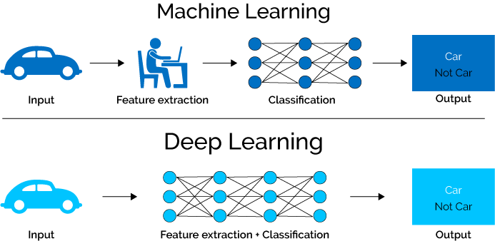
Before starting lets have a look at the two different terms which are Machine Learning and Deep Learning which are closely related. The following diagram show pictorially the key difference:
With Machine Learning the approach works like the top half of the picture above. You would have to design a feature extraction algorithm which generally involved a lot of heavy mathematics (complex design), wasn’t very efficient, and didn’t perform too well at all (accuracy level just wasn’t suitable for real-world applications). After doing all of that you would also have to design a whole classification model to classify your input given the extracted features.
With Deep Learning networks we can perform feature extraction and classification in one shot, which means we only have to design one model. This also means that with have a lot more layers (usually) and parameters to refine our model to an optimal point.
Machine Learning
- + Good results
- + Quick to train
- - Need to try different features and classifiers to achieve best results
- - Accuracy plateaus
Deep Learning
- + Learns features and classifiers automatically
- + Accuracy is unlimited
- - Requires very large data sets
- - Computationally intensive / expensive
Introduction to Python and its libraries
Python is a general-purpose high level programming language that is widely used in data science and for producing deep learning algorithms. This brief tutorial introduces Python and its libraries like Numpy, skimage, TensorFlow, Keras.
Deep structured learning or hierarchical learning or deep learning in short is part of the family of machine learning methods which are themselves a subset of the broader field of Artificial Intelligence.
Machine learning deals with a wide range of concepts. The concepts are listed below −
- supervised
- unsupervised
- reinforcement learning
- linear regression
- cost functions
- overfitting
- under-fitting
- hyper-parameter, etc.
In supervised learning, we learn to predict values from labelled data. One ML technique that helps here is classification, where target values are discrete values; for example, cats and dogs. Another technique in machine learning that could come of help is regression. Regression works on the target values. The target values are continuous values; for example, the stock market data can be analysed using Regression.
Introduction to Neural Network
A typical neural network has anything from a few dozen to hundreds, thousands, or even millions of artificial neurons called units arranged in a series of layers, each of which connects to the layers on either side. Some of them, known as input units, are designed to receive various forms of information from the outside world that the network will attempt to learn about, recognise, or otherwise process. Other units sit on the opposite side of the network and signal how it responds to the information it's learned; those are known as output units. In between the input units and output units are one or more layers of hidden units, which, together, form most of the artificial brain. Most neural networks are fully connected, which means each hidden unit and each output unit is connected to every unit in the layers either side. The connections between one unit and another are represented by a number called a weight, which can be either positive (if one unit excites another) or negative (if one unit suppresses or inhibits another). The higher the weight, the more influence one unit has on another. (This corresponds to the way actual brain cells trigger one another across tiny gaps called synapses.)
Information flows through a neural network in two ways. When it's learning (being trained) or operating normally (after being trained), patterns of information are fed into the network via the input units, which trigger the layers of hidden units, and these in turn arrive at the output units. This common design is called a feedforward network. Not all units "fire" all the time. Each unit receives inputs from the units to its left, and the inputs are multiplied by the weights of the connections they travel along. Every unit adds up all the inputs it receives in this way and (in the simplest type of network) if the sum is more than a certain threshold value, the unit "fires" and triggers the units it's connected to (those on its right).
For a neural network to learn, there has to be an element of feedback involved—just as children learn by being told what they're doing right or wrong. In fact, we all use feedback, all the time. Think back to when you first learned to play a game like ten-pin bowling. As you picked up the heavy ball and rolled it down the alley, your brain watched how quickly the ball moved and the line it followed, and noted how close you came to knocking down the skittles. Next time it was your turn, you remembered what you'd done wrong before, modified your movements accordingly, and hopefully threw the ball a bit better. So you used feedback to compare the outcome you wanted with what actually happened, figured out the difference between the two, and used that to change what you did next time ("I need to throw it harder," "I need to roll slightly more to the left," "I need to let go later," and so on). The bigger the difference between the intended and actual outcome, the more radically you would have altered your moves.
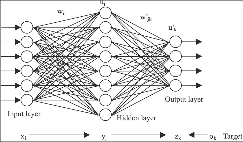
Below shows a neural network example with inputs on the left, a hidden layer, and an output layer. In code we will try to mimic this theory.
- input layer: brings the initial data into the system for further processing by subsequent layers of artificial neurons.
- hidden layer: a layer in between input layers and output layers, where artificial neurons take in a set of weighted inputs and produce an output through an activation function.
- output layer: the last layer of neurons that produces given outputs for the program.
An artificial neural network consists of artificial neurons or processing elements and is organised in three interconnected layers: input, hidden that may include more than one layer, and output.
The input layer contains input neurons that send information to the hidden layer. The hidden layer sends data to the output layer. Every neuron has weighted inputs (synapses), an activation function (defines the output given an input), and one output. Synapses are the adjustable parameters that convert a neural network to a parameter system.
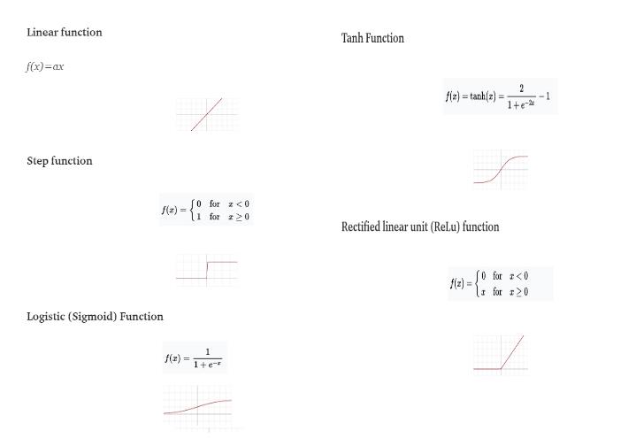
The weighted sum of the inputs produces the activation signal that is passed to the activation function to obtain one output from the neuron. The commonly used activation functions are linear, step, sigmoid, tanh, and rectified linear unit (ReLu) functions.
Neural networks learn things in exactly the same way, typically by a feedback process called back-propagation (sometimes abbreviated as "backprop"). This involves comparing the output a network produces with the output it was meant to produce and using the difference between them to modify the weights of the connections between the units in the network, working from the output units through the hidden units to the input units—going backward, in other words. In time, back-propagation causes the network to learn, reducing the difference between actual and intended output to the point where the two exactly coincide, so the network figures things out exactly as it should.
Gradient Descent
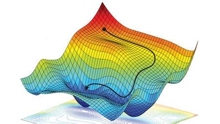
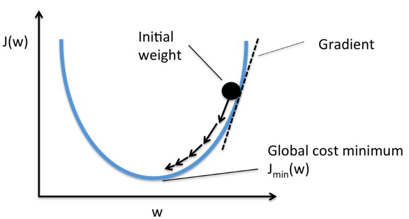
Gradient descent has an analogy of looking for the easiest way down a mountain side, you're going to look for the most gentle way down. In reality it is a highly mathematical function but for most programmers this is hidden.
From the programming point of view gradient descent is an iterative method. We start with some set of values for our model parameters (weights and biases), and improve them slowly.
To improve a given set of weights, we try to get a sense of the value of the cost function (described below) for weights similar to the current weights (by calculating the gradient). Then we move in the direction which reduces the cost function.
By repeating this step thousands of times, we’ll continually minimise our cost function.
On gradients and gradient learning algorithms, the main optimisation technique used to fit neural network weights to training data-sets.
This includes the important distinction between batch and stochastic gradient descent, and approximations via mini-batch gradient descent, today all simply referred to as stochastic gradient descent.
- Batch Gradient Descent. Gradient is estimated using all examples in the training data set.
- Stochastic (Online) Gradient Descent. Gradient is estimated using subsets of samples in the training data set.
- Mini-Batch Gradient Descent. Gradient is estimated using each single pattern in the training data set.
The mini-batch variant is offered as a way to achieve the speed of convergence offered by stochastic gradient descent with the improved estimate of the error gradient offered by batch gradient descent.
- Larger batch sizes slow down convergence.
- Smaller batch sizes offer a regularising effect due to the introduction of statistical noise in the gradient estimate.
Loss and accuracy
Deep learning neural networks are trained using the stochastic gradient descent optimisation algorithm.
As part of the optimisation algorithm, the error for the current state of the model must be estimated repeatedly. This requires the choice of an error function, conventionally called a loss function, that can be used to estimate the loss of the model so that the weights can be updated to reduce the loss on the next evaluation.
The maths function Mean Square Error (MSE) is the most commonly used regression loss function. MSE is the sum of squared distances between our target variable and predicted values.
Neural network models learn a mapping from inputs to outputs from examples and the choice of loss function must match the framing of the specific predictive modelling problem, such as classification or regression. Further, the configuration of the output layer must also be appropriate for the chosen loss function.
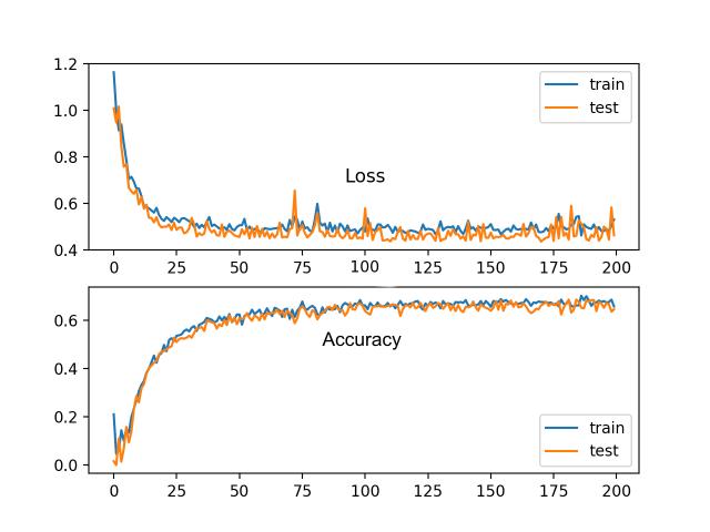
As we keep applying training data to our neural network model we need to measure how close we are achieving our goal, with a suitable model we should describe something like the following:
Tensorflow and Keras Libraries
Tensorflow
Google's TensorFlow is a python library. This library is a great choice for building commercial grade deep learning applications.
TensorFlow grew out of another library DistBelief V2 that was a part of Google Brain Project. This library aims to extend the portability of machine learning so that research models could be applied to commercial-grade applications.
Much like the Theano library, TensorFlow is based on computational graphs where a node represents persistent data or math operation and edges represent the flow of data between nodes, which is a multidimensional array or tensor; hence the name TensorFlow
The output from an operation or a set of operations is fed as input into the next.
Even though TensorFlow was designed for neural networks, it works well for other nets where computation can be modelled as data flow graph.
TensorFlow also uses several features from Theano such as common and sub-expression elimination, auto differentiation, shared and symbolic variables.
Different types of deep nets can be built using TensorFlow like convolutional nets, Autoencoders, RNTN, RNN, RBM, DBM/MLP and so on.
However, there is no support for hyper parameter configuration in TensorFlow. For this functionality, we can use Keras.
Keras
Keras is a powerful easy-to-use Python library for developing and evaluating deep learning models.
It has a minimalist design that allows us to build a net layer by layer; train it, and run it.
It wraps the efficient numerical computation libraries Theano and TensorFlow and allows us to define and train neural network models in a few short lines of code.
It is a high-level neural network API, helping to make wide use of deep learning and artificial intelligence. It runs on top of a number of lower-level libraries including TensorFlow, Theano,and so on. Keras code is portable; we can implement a neural network in Keras using Theano or TensorFlow as a back ended without any changes in code.
mnist dataset
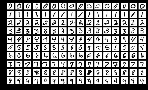
The MNIST database (Modified National Institute of Standards and Technology database) is a large database of handwritten digits that is commonly used for training various image processing systems. The database is also widely used for training and testing in the field of machine learning. It was created by "re-mixing" the samples from NIST's original datasets. The creators felt that since NIST's training dataset was taken from American Census Bureau employees, while the testing dataset was taken from American high school students, it was not well-suited for machine learning experiments. Furthermore, the black and white images from NIST were normalized to fit into a 28x28 pixel bounding box and anti-aliased, which introduced grayscale levels.
The MNIST database contains 60,000 training images and 10,000 testing images. Half of the training set and half of the test set were taken from NIST's training dataset, while the other half of the training set and the other half of the test set were taken from NIST's testing dataset. There have been a several scientific papers on attempts to achieve the lowest error rate; one paper, using a hierarchical system of convolutional neural networks, manages to get an error rate on the MNIST database of 0.23%. The original creators of the database keep a list of some of the methods tested on it. In their original paper, they use a support vector machine to get an error rate of 0.8%. An extended dataset similar to MNIST called EMNIST has been published in 2017, which contains 240,000 training images, and 40,000 testing images of handwritten digits and characters
This classic dataset is the ideal for neural nets since it has image data and the correct answer to compare our test network.
We will now look at three different ways of running this network with different methods:
#
# Described neural net builder program
# Darren Bird - HPC Viper Team
#
import tensorflow as tf
from tensorflow.examples.tutorials.mnist import input_data

mnist = input_data.read_data_sets("/tmp/data/", one_hot=True)

n_nodes_hl1= 30
n_nodes_hl2= 20


n_classes = 10
batch_size = 100

# height x width
# x is 784 is a flat array of a 28x28 pixel image
#

x = tf.placeholder('float',[None, 784]);
y = tf.placeholder('float');

# Limit parallelism on multicore system for fair play

config = tf.ConfigProto()
config.intra_op_parallelism_threads = 1
config.inter_op_parallelism_threads= 1

# This builds the computational graph up, but does not execute it here!

def neural_network_model(data):

        hidden_1_layer = {'weights':tf.Variable(tf.random_normal([784, n_nodes_hl1])),
                'biases':tf.Variable(tf.random_normal([n_nodes_hl1]))}

        hidden_2_layer = {'weights':tf.Variable(tf.random_normal([n_nodes_hl1, n_nodes_hl2])),
                'biases':tf.Variable(tf.random_normal([n_nodes_hl2]))}

        output_layer = {'weights':tf.Variable(tf.random_normal([n_nodes_hl2, n_classes])),
                'biases':tf.Variable(tf.random_normal([n_classes]))}

        # (input_data * weights) + biases

        l1 = tf.add(tf.matmul(data, hidden_1_layer['weights']), hidden_1_layer['biases'])
        l1 = tf.nn.relu(l1)

        l2 = tf.add(tf.matmul(l1, hidden_2_layer['weights']), hidden_2_layer['biases'])
        l2 = tf.nn.relu(l2)

        output = tf.matmul(l2, output_layer['weights']) + output_layer['biases']

        return output

def train_neural_network(x):

        prediction = neural_network_model(x)

        # print ("prediction " + prediction)

        cost = tf.reduce_mean( tf.nn.softmax_cross_entropy_with_logits(logits=prediction,
                labels=y) )

        # print ("cost " + cost)

        # learning_rate = 0.001 - Adam optimizer

        optimizer = tf.train.AdamOptimizer().minimize(cost)

        # cycles feed forward + backprop
        hm_epochs = 40

        # run computational graph

        with tf.Session(config=config) as sess:
                sess.run(tf.global_variables_initializer() )

                for epoch in range(hm_epochs):
                        epoch_loss = 0

                        for _ in range(int(mnist.train.num_examples/batch_size)):
                                epoch_x, epoch_y = mnist.train.next_batch(batch_size)

                                _, c = sess.run([optimizer, cost], feed_dict = {x: epoch_x, y: epoch_y})

                                epoch_loss += c
                        print('Epoch', epoch, ' completed out of ', hm_epochs, ' loss:',epoch_loss)

                correct = tf.equal(tf.argmax(prediction,1), tf.argmax(y,1))

                accuracy = tf.reduce_mean(tf.cast(correct, 'float'))

                print('Accuracy:',accuracy.eval( {x:mnist.test.images, y: mnist.test.labels} ))

        return

train_neural_network(x)
Program output
Extracting /tmp/data/train-images-idx3-ubyte.gz
Extracting /tmp/data/train-labels-idx1-ubyte.gz
Extracting /tmp/data/t10k-images-idx3-ubyte.gz
Extracting /tmp/data/t10k-labels-idx1-ubyte.gz
Epoch 0  completed out of  40  loss: 10784.182388782501
Epoch 1  completed out of  40  loss: 1482.2316706180573
Epoch 2  completed out of  40  loss: 1263.2460134029388
Epoch 3  completed out of  40  loss: 1169.1023557186127
.
.
.
Epoch 37  completed out of  40  loss: 101.28223147243261
Epoch 38  completed out of  40  loss: 98.11811654642224
Epoch 39  completed out of  40  loss: 95.58086830750108
Accuracy: 0.9345
By running the above code you can see the computer going through the images in batches.
epoch_x, epoch_y = mnist.train.next_batch(batch_size)
It compares the outputs of our neural network with the actual outputs. Each time we try and minimise how far we are away from that answer
optimizer = tf.train.AdamOptimizer().minimize(cost)
By changing those neural network weights in relation to the outputs which we measure using a mathematical function called gradient descent and changing those weights by a process called back propagation.
_, c = sess.run([optimizer, cost], feed_dict = {x: epoch_x, y: epoch_y})
Same mnist data but more complex network
This uses the library KERAS on top of the TENSORFLOW library to simplify the construction of a more complex model. This can be seen in the following code below where each line defines a complete layer of the model:
model = Sequential()
model.add(Conv2D(32, kernel_size=(3, 3),
                 activation='relu',
                 input_shape=input_shape))
model.add(Conv2D(64, (3, 3), activation='relu'))
model.add(MaxPooling2D(pool_size=(2, 2)))
model.add(Dropout(0.25))
model.add(Flatten())
model.add(Dense(128, activation='relu'))
model.add(Dropout(0.5))
model.add(Dense(num_classes, activation='softmax'))
Keras code example
'''Trains a simple convnet on the MNIST dataset.
Gets to 99.25% test accuracy after 12 epochs
(there is still a lot of margin for parameter tuning).
'''

from __future__ import print_function
import keras
from keras.datasets import mnist
from keras.models import Sequential
from keras.layers import Dense, Dropout, Flatten
from keras.layers import Conv2D, MaxPooling2D
from keras import backend as K
import time

K.set_session(K.tf.Session(config=K.tf.ConfigProto(intra_op_parallelism_threads=1, inter_op_parallelism_threads=1)))
start_time = time.time()

batch_size = 128
num_classes = 10
epochs = 12

# input image dimensions
img_rows, img_cols = 28, 28

# the data, shuffled and split between train and test sets
(x_train, y_train), (x_test, y_test) = mnist.load_data()

if K.image_data_format() == 'channels_first':
    x_train = x_train.reshape(x_train.shape[0], 1, img_rows, img_cols)
    x_test = x_test.reshape(x_test.shape[0], 1, img_rows, img_cols)
    input_shape = (1, img_rows, img_cols)
else:
    x_train = x_train.reshape(x_train.shape[0], img_rows, img_cols, 1)
    x_test = x_test.reshape(x_test.shape[0], img_rows, img_cols, 1)
    input_shape = (img_rows, img_cols, 1)

x_train = x_train.astype('float32')
x_test = x_test.astype('float32')
x_train /= 255
x_test /= 255
print('x_train shape:', x_train.shape)
print(x_train.shape[0], 'train samples')
print(x_test.shape[0], 'test samples')

# convert class vectors to binary class matrices
y_train = keras.utils.to_categorical(y_train, num_classes)
y_test = keras.utils.to_categorical(y_test, num_classes)

# build neural net layers up, does not run them yet!

model = Sequential()
model.add(Conv2D(32, kernel_size=(3, 3),
                 activation='relu',
                 input_shape=input_shape))
model.add(Conv2D(64, (3, 3), activation='relu'))  #------ try changing activation to 'sigmoid'
model.add(MaxPooling2D(pool_size=(2, 2)))
model.add(Dropout(0.25))                      #---------- try changing these between 0 - 1.0
model.add(Flatten())
model.add(Dense(128, activation='relu'))      #---------- sigmoid
model.add(Dropout(0.5))                       #---------- try changing these between 0 - 1.0, then RUN
model.add(Dense(num_classes, activation='softmax'))

# make the graph and now run it with the data

model.compile(loss=keras.losses.categorical_crossentropy,
              optimizer=keras.optimizers.Adadelta(),
              metrics=['accuracy'])

model.fit(x_train, y_train,
          batch_size=batch_size,
          epochs=epochs,
          verbose=1,
          validation_data=(x_test, y_test))
score = model.evaluate(x_test, y_test, verbose=0)

# print out the answers

print('Test loss:', score[0])
print('Test accuracy:', score[1])

print("--- %s seconds ---" % (time.time() - start_time))
Keras code example (more refined again)
'''Trains a simple deep NN on the MNIST dataset.
Gets to 98.40% test accuracy after 20 epochs(there is *a lot* of margin for parameter tuning).
'''

from __future__ import print_function
import keras
from keras.datasets import mnist
from keras.models import Sequential
from keras.layers import Dense, Dropout
from keras.optimizers import RMSprop
from keras import backend as K
import time

# Don't change this line
K.set_session(K.tf.Session(config=K.tf.ConfigProto(intra_op_parallelism_threads=10, inter_op_parallelism_threads=10)))

start_time = time.time()
batch_size = 128
num_classes = 10
epochs = 20

# the data, shuffled and split between train and test sets
(x_train, y_train), (x_test, y_test) = mnist.load_data()

x_train = x_train.reshape(60000, 784)
x_test = x_test.reshape(10000, 784)
x_train = x_train.astype('float32')
x_test = x_test.astype('float32')
x_train /= 255
x_test /= 255
print(x_train.shape[0], 'train samples')
print(x_test.shape[0], 'test samples')

# convert class vectors to binary class matrices
y_train = keras.utils.to_categorical(y_train, num_classes)
y_test = keras.utils.to_categorical(y_test, num_classes)

# build layers up

model = Sequential()

model.add(Dense(1024, activation='relu', input_shape=(784,)))
model.add(Dropout(0.99))
model.add(Dense(10, activation='relu'))
model.add(Dropout(0.85))
model.add(Dense(num_classes, activation='sigmoid'))

model.summary()

# make computational graph and run it with data

model.compile(loss='categorical_crossentropy',
              optimizer=RMSprop(),
              metrics=['accuracy'])

history = model.fit(x_train, y_train,
                    batch_size=batch_size,
                    epochs=epochs,
                    verbose=1,
                    validation_data=(x_test, y_test))
score = model.evaluate(x_test, y_test, verbose=0)

print('Test loss:', score[0])
print('Test accuracy:', score[1])
print("--- %s seconds ---" % (time.time() - start_time))
Setting Hyperparameters
Initial Learning Rate. The proportion that weights are updated; 0.01 is a good start. Mini-batch Size. Number of samples used to estimate the gradient; 32 is a good start. Training Iterations. Number of updates to the weights; set large and use early stopping. The learning rate is presented as the most important parameter to tune. Although a value of 0.01 is a recommended starting point, dialing it in for a specific dataset and model is required.
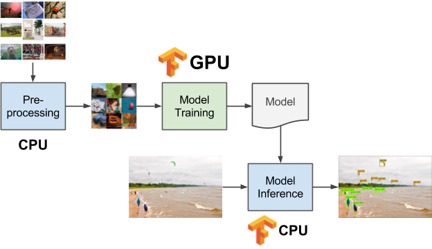
Using a GPU to run a neural network
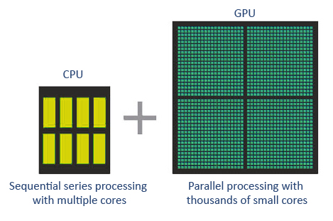
GPUs are so fast because they are so efficient for matrix multiplication and convolution ideal for Deep learning. They are not better than CPUs which are a much more general-purpose processing unit, CPUs can perform out of order computations and have large caches (L1, L2 and L3) which take up large amount of silicon. GPUs are very good at processing large array data in one go as they are predominantly small processors and shared memory.
Although GPUs are very fast, one disadvantage is moving the data from CPU memory (host) to the GPU (device), and backwards after processing.
Now the GPUs on the university's supercomputer are NVidia K40 which have 2880 streaming processors which makes it ideal for processing a large amount of data in one go. Although CPU are very good, they are latency optimized while GPUs are bandwidth optimized. You can visualize this as a CPU being a Ferrari and a GPU being a big truck. The task of both is to pick up packages from a random location A and to transport those packages to another random location B. The CPU (Ferrari) can fetch some memory (packages) in your RAM quickly while the GPU (big truck) is slower in doing that (much higher latency). However, the CPU (Ferrari) needs to go back and forth many times to do its job.
Nearly all production Deep model learning is done on GPU accelerators.
Summary
Deep learning has produced good results for a few applications such as computer vision, language translation, image captioning, audio transcription, molecular biology, speech recognition, natural language processing, self-driving cars, brain tumour detection, real-time speech translation, music composition, automatic game playing and so on.
Deep learning is the next big leap after machine learning with a more advanced implementation. Currently, it is heading towards becoming an industry standard bringing a strong promise of being a game changer when dealing with raw unstructured data.
Deep learning is currently one of the best solution providers fora wide range of real-world problems. Developers are building AI programs that, instead of using previously given rules, learn from examples to solve complicated tasks. With deep learning being used by many data scientists, deeper neural networks are delivering results that are ever more accurate.
The idea is to develop deep neural networks by increasing the number of training layers for each network; machine learns more about the data until it is as accurate as possible. Developers can use deep learning techniques to implement complex machine learning tasks, and train AI networks to have high levels of perceptual recognition.
Viper Development Environments
There are the following development environments already part of our HPC
- Python 3.5 with Tensorflow (and Keras), and theano.
- C/C++/Fortran with CUDA GPU programming.
- PGI compiler with openACC programming for C and Fortran.
- Matlab with deep learning libraries.
Useful links for further reading
If you're interested in looking into this subject have a look at the following links:
Tutorials
- https://medium.com/@erikhallstrm/hello-world-rnn-83cd7105b767 https://www.datacamp.com/community/tutorials/tensorflow-tutorial * * * *
- https://cs224d.stanford.edu/lectures/CS224d-Lecture7.pdf https://www.toptal.com/machine-learning/tensorflow-machine-learning-tutorial *
- https://pythonprogramming.net/tensorflow-introduction-machine-learning-tutorial/
- https://www.nvidia.com/en-gb/deep-learning-ai/education/
Tensorflow
Keras
Software repositories
- https://github.com/Hvass-Labs/TensorFlow-Tutorials https://github.com/aymericdamien/TensorFlow-Examples
- https://github.com/tensorflow/tensorflow/tree/master/tensorflow/examples/tutorials
| |

